Posts published in “SP”

花花酱 Amortized Analysis 均摊分析 SP7

By zxi on September 17, 2018

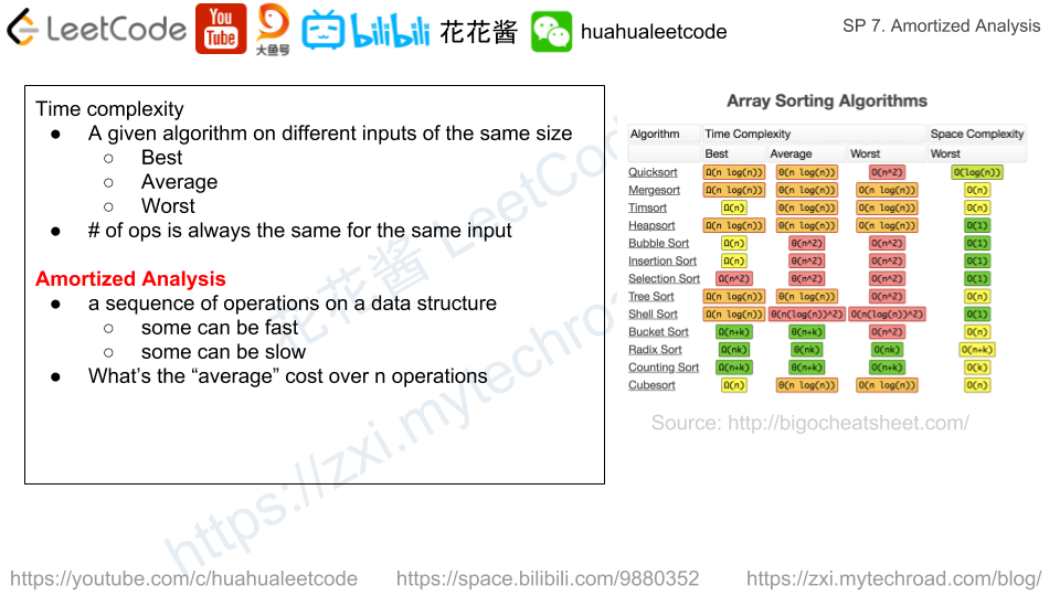
Amortized Analysis

Amortized analysis can help us understand the actual cost of n operations on a data structure. Since some operations can be really fast e.g. O(1), but some operations can be really slow e.g. O(n). We could say the time complexity of that operation is O(n). However, it does not reflect the actual performance. And turns out, we can prove that certain operations have an amortized cost of O(1) while they can take O(n) in the worst case.

均摊分析可以帮助我们了解对一个数据结构进行n次操作的真实代价。对于相同的操作，有时候可以非常快，例如在O(1)时间内完成，而有时候则需要O(n)。我们当然可以说这个操作最坏情况下的时间复杂度是O(n)，但是这并不能真实反映它的实际复杂度。通过均摊分析，我们可以证明，尽管有些操作在最坏情况下是O(n)的时间复杂度，但是均摊下来只需要O(1)。

Dynamic Array

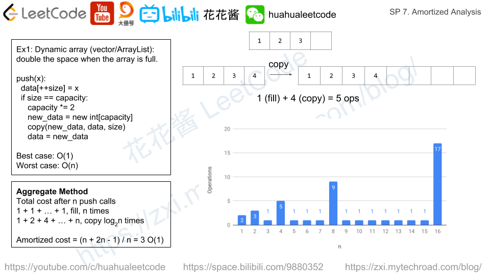
dynamic array doubles its size when it’s full which could take O(i) time where i is the number of elements in the array. Otherwise just store the element which only cost O(1). We can use aggregate method to compute the amortized cost of dynamic array.

动态数组在容量满时将容量翻翻，这一步需要O(i)时间，i是当前数组中的元素个数。如果没有满，只需要将元素存储下来即可，只需要花费O(1)时间。我们可以使用聚合法来计算均摊成本。

((1 + 1) + (1 + 2) + (1) + (1 + 4) + (1) + (1) + (1) + (1+8) + … + (1+n)) / n, assuming n is 2^k.

= (1 * n + (1 + 2 + 4 + 8 + … + n)) / n = (n + 2n – 1) / n = 3. O(1)

C++

#include <iostream>

#include <algorithm>

using namespace std;

class DynamicArray {

public:

DynamicArray() {

data_ = new int[1];

capcity_ = 1;

}

void add(int x) {

data_[size_++] = x;

++total_cost_;

if (size_ == capcity_) {

capcity_ *= 2;

total_cost_ += size_;

int* new_data = new int[capcity_];

copy(data_, data_ + size_, new_data);

swap(new_data, data_);

delete [] new_data;

}

int totalCost() const { return total_cost_; }

private:

int total_cost_ = 0;

int size_ = 0;

int capcity_;

int* data_;

};

int main() {

DynamicArray arr;

for (int i = 1; i <= 16; ++i) {

arr.add(i);

cout << i << " average cost: " << arr.totalCost() / static_cast<float>(i) << endl;

}

Output

1 average cost: 2

2 average cost: 2.5

3 average cost: 2

4 average cost: 2.75

5 average cost: 2.4

6 average cost: 2.16667

7 average cost: 2

8 average cost: 2.875

9 average cost: 2.66667

10 average cost: 2.5

11 average cost: 2.36364

12 average cost: 2.25

13 average cost: 2.15385

14 average cost: 2.07143

15 average cost: 2

16 average cost: 2.9375

[Finished in 0.4s]

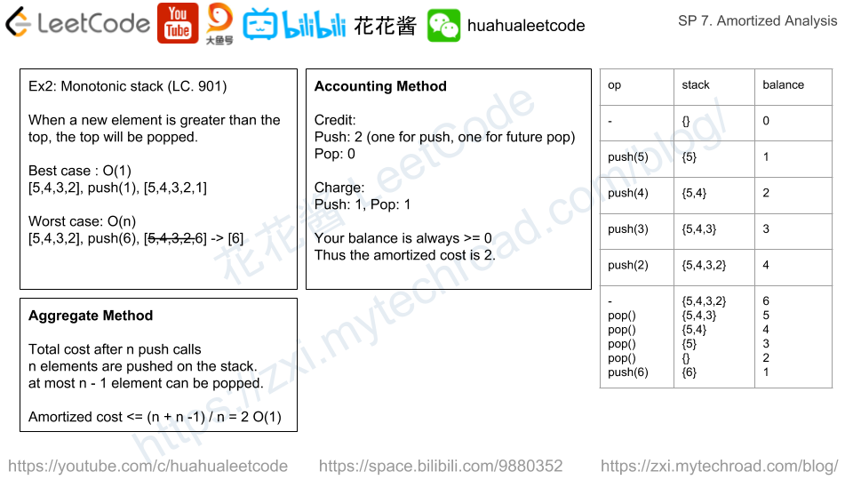
Monotonic Stack

例子2: 单调栈

往单调栈push一个元素的时候，会删除上所有小于等于它的元素。这步操作在最优情况下是O(1)时间，如果它比栈顶元素要小。在最坏情况下是O(i)时间，栈上有i个元素，它比这i个元素都要大，所以一共要pop i次。

聚合法：

由于每个元素都会被push到栈上去1次，最多会被pop1次，所以总的操作数 <= 2n。 2n / n = 2 O(1)。

会计法：

每次push之前先存k块钱，k=2, 一块钱用于push自己，一块钱留着用于pop自己。

push的时候扣除1块钱，pop的时候再扣除1块钱。但不管怎样，我的账户上的钱永远>=0。这样我们可以说push的均摊成本是k=2。同样是O(1)，尽管它的worst case是O(n)。

C++

#include <iostream>

#include <algorithm>

#include <stack>

using namespace std;

class MonotonicStack {

public:

void push(int x) {

while (!data_.empty() && x > data_.top()) {

this->pop();

}

++total_cost_;

data_.push(x);

}

int pop() {

++total_cost_;

int t = data_.top();

data_.pop();

return t;

}

int totalCost() const { return total_cost_; }

private:

int total_cost_ = 0;

stack<int> data_;

};

int main() {

srand(1);

MonotonicStack s;

for (int i = 1; i <= 32; ++i) {

s.push(rand());

cout << i << " average cost: " << s.totalCost() / static_cast<float>(i) << endl;

}

Output

1 average cost: 1

2 average cost: 1.5

3 average cost: 1.66667

4 average cost: 1.5

5 average cost: 1.6

6 average cost: 1.5

7 average cost: 1.42857

8 average cost: 1.75

9 average cost: 1.77778

10 average cost: 1.9

11 average cost: 1.81818

12 average cost: 1.83333

13 average cost: 1.84615

14 average cost: 1.78571

15 average cost: 1.8

16 average cost: 1.8125

17 average cost: 1.82353

18 average cost: 1.77778

19 average cost: 1.78947

20 average cost: 1.75

21 average cost: 1.80952

22 average cost: 1.86364

23 average cost: 1.82609

24 average cost: 1.91667

25 average cost: 1.88

26 average cost: 1.84615

27 average cost: 1.81481

28 average cost: 1.85714

29 average cost: 1.82759

30 average cost: 1.86667

31 average cost: 1.90323

32 average cost: 1.875

[Finished in 0.5s]

Mentioned Problems

花花酱 Time/Space Complexity of Recursion Functions SP4

By zxi on February 7, 2018

How to analyze the time and space complexity of a recursion function?

如何分析一个递归函数的时间/空间复杂度？

We can answer that using master theorem or induction in most of the cases.

在大部分时候我们可以使用主方法和数学归纳法来进行解答。

First of all, we need to write down the recursion relation of a function.

首先我们要写出一个函数的递归表达式。

def func(n):

if n < 0: return 1

return func(n/2) + func(n/2)

Let’s use T(n) to denote the running time of func with input size of n.

让我们用T(n)来表示func函数在输入规模为n的运行时间。

Then we have：

那么我们有：

T(n) = 2*T(n/2) + O(1)

a = 2, b = 2, c_crit = logb(a) = 1, f(n) = n^c, c = 0.

c < c_crit, apply master theorem case 1:

根据主方法第一条我们得到

T(n) = Θ(n^c_crit) = Θ(n)

Let’s look at another example:

def func(n):

if n < 0: return 1

s = 0

for i in range(n):

s += i

return s + func(n/2) + func(n/2)

T(n) = 2*T(n/2) + O(n)

a = 2, b = 2, c_crit = logb(a) = 1, f(n) = n^c, c = 1,

c = c_crit, apply master theorem case 2:

根据主方法第二条我们得到

T(n) =Θ(n^c_crit * (logn)^1)) = Θ(nlogn)

Cheatsheet

Equation	Time	Space	Examples
T(n) = 2*T(n/2) + O(n)	O(nlogn)	O(logn)	quick_sort
T(n) = 2*T(n/2) + O(n)	O(nlogn)	O(n + logn)	merge_sort
T(n) = T(n/2) + O(1)	O(logn)	O(logn)	Binary search
T(n) = 2*T(n/2) + O(1)	O(n)	O(logn)	Binary tree traversal
T(n) = T(n-1) + O(1)	O(n)	O(n)	Binary tree traversal
T(n) = T(n-1) + O(n)	O(n^2)	O(n)	quick_sort(worst case)
T(n) = n * T(n-1)	O(n!)	O(n)	permutation
T(n) = T(n-1)+T(n-2)+…+T(1)	O(2^n)	O(n)	combination

For recursion with memorization:

Time complexity: |# of subproblems| * |exclusive running time of a subproblem|

Example 1:

def fib(n):

if n < 1: return 1

if m[n]: return m[n]

m[n] = fib(n - 1) + fib(n - 2)

return m[n]

To solve fib(n), there are n subproblems fib(0), fib(1), …, fib(n)

each sub problem takes O(1) to solve

Time complexity: O(n)

Space complexity: O(n) + O(n) * O(1) = O(n)

Example 2:

LC 741 Cherry Pickup

dp(x1, y1, x2):

if min(x1, y1, x2) < 0: return 0

if m[x1][y1][x2]: return m[x1][y1][x2]

ans = max(dp(x1 - 1, y1, x2 - 1),

dp(x1, y1 - 1, x2),

dp(x1, y1 - 1, x2 - 1),

dp(x1 - 1, y1, x2))

m[x1][y1][x2] = ans

return m[x1][y1][x2]

To solve dp(n, n, n), there are n^3 subproblems

each subproblem takes O(1) to solve

Max recursion depth O(n)

Time complexity: O(n^3) * O(1) = O(n^3)

Space complexity: O(n^3) + O(n) * O(1) = O(n^3)

Example 3:

LC 312: Burst Balloon

dp(i, j):

if m[i][j]: return m[i][j]

for k in range(i, j + 1):

ans = max(ans, dp(i, k - 1) + C + dp(k + 1, j))

m[i][j] = ans

return m[i][j]

To solve dp(0, n), there are n^2 subproblems dp(0, 0), dp(0, 1), …, dp(n-1, n)

each subproblem takes O(n) to solve

Max recursion depth O(n)

Time complexity: O(n^2) * O(n) = O(n^3)

Space complexity: O(n^2) + O(n) * O(1) = O(n^2)

Slides:

花花酱 Fenwick Tree / Binary Indexed Tree / 树状数组 SP3

By zxi on January 3, 2018

本期节目中我们介绍了Fenwick Tree/Binary Indexed Tree/树状数组的原理和实现以及它在leetcode中的应用。
In this episode, we will introduce Fenwick Tree/Binary Indexed Tree, its idea and implementation and show its applications in leetcode.

Fenwick Tree is mainly designed for solving the single point update range sum problems. e.g. what’s the sum between i-th and j-th element while the values of the elements are mutable.

Init the tree (include building all prefix sums) takes O(nlogn)

Update the value of an element takes O(logn)

Query the range sum takes O(logn)

Space complexity: O(n)

Applications:

Implementation:

C++

class FenwickTree {

public:

FenwickTree(int n): sums_(n + 1, 0) {}

void update(int i, int delta) {

while (i < sums_.size()) {

sums_[i] += delta;

i += lowbit(i);

}

int query(int i) const {

int sum = 0;

while (i > 0) {

sum += sums_[i];

i -= lowbit(i);

}

return sum;

}

private:

static inline int lowbit(int x) {

return x & (-x);

}

vector<int> sums_;

};

Java

class FenwickTree {

int sums_[];

public FenwickTree(int n) {

sums_ = new int[n + 1];

}

public void update(int i, int delta) {

while (i < sums_.length) {

sums_[i] += delta;

i += i & -i;

}

public int query(int i) {

int sum = 0;

while (i > 0) {

sum += sums_[i];

i -= i & -i;

}

return sum;

}

Python3

class FenwickTree:

def __init__(self, n):

self._sums = [0 for _ in range(n + 1)]

def update(self, i, delta):

while i < len(self._sums):

self._sums[i] += delta

i += i & -i

def query(self, i):

s = 0

while i > 0:

s += self._sums[i]

i -= i & -i

return s

Applications

花花酱 LeetCode Input Size V.S. Time Complexity SP2

By zxi on December 28, 2017

本期节目介绍了输入数据规模和时间复杂度上限的关系，可以通过数据规模推算使用算法的类型。

< 10: O(n!) permutation
< 15: O(2^n) combination
< 50: O(n^4) DP
< 200: O(n^3) DP, all pairs shortest path
< 1,000: O(n^2) DP, all pairs, dense graph
< 1,000,000: O(nlogn), sorting-based (greedy), heap, divide & conquer
< 1,000,000: O(n), DP, graph traversal / topological sorting (V+E), tree traversal
< INT_MAX: O(sqrt(n)), prime, square sum
< INT_MAX: O(logn), binary search
< INT_MAX: O(1) Math

Posts published in “SP”

花花酱 Amortized Analysis 均摊分析 SP7

Amortized Analysis

Dynamic Array

C++

Output

Monotonic Stack

C++

Output

Related Problem

花花酱 SP5 Binary Search

Mentioned Problems

花花酱 Time/Space Complexity of Recursion Functions SP4

花花酱 Fenwick Tree / Binary Indexed Tree / 树状数组 SP3

C++

Java

Python3

Applications

花花酱 LeetCode Input Size V.S. Time Complexity SP2